Basic Workflow

After setting up the required dependencies and reference templates, users may begin segmenting 3D mandibles from an input raw CT image (test scan).

What follows is a list of all commands used in the SAMS pipeline. Variable names/values/files needed to be modified by users are enclosed between < … >.

For example, below is a command applying threshold to a mandible image

Example

$ fslmaths <input_mandible_image> -thr <user_decided_threshold_value> -uthr 3000 <output_thresholded_mandible_image>

where

• fslmaths is the executing function,

• <input_mandible_image>, as stated in the variable name, refers to the file of the input mandible image, so users should replace this value with the filename (eg: mandibleA.nii),

• thr is the setting to the executing function, in this case the value following this will set the value to the minimum threshold,

• <user_decided_threshold_value> is a numerical value the user assigns to be the minimum threshold,

• uthr is also the setting to the executing function, stands for “upper threshold”, the value following this will set the value to the maximum / upper threshold limit,

• 3000 is the upper threshold limit,

• <output_thresholded_mandible_image>, as stated in the variable name, this will be the output of the above setting, users should enter the desired output filename here (eg: mandibleThresholded.nii)

Note

Refer to related documentations of functions and commands described in this documentation for detailed explanation.

Input Preparation

Before starting the SAMS pipeline, the desired input files should be converted from DICOM series into Analyze75 file format [.hdr/.img] or equivalent format.

In Analyze 12.0, user needs to inspect the scan and collect the threshold needed to remove all non-osseous tissues from the 3D renderings.

If an alternative software is used for inspection and threshold collection, the input file can also be saved as NIfTI file format [.nii or .nii.gz].

The following pre-processing step accepts both Analyze75 and NIfTI file format as the input test scan.

Pre-processing

In pre-processing, the input test scan will be inspected by user to:

1. Find a threshold value in Hounsfield Unit (HU) that provides best quality of the mandible.

2. Find the minimal enclosing box that contains the mandible.

In Analyze 12.0, the threshold value is determined by adjusting for the minimum threshold that will render a 3D mandible free of all non-osseous tissue. Typical threshold range between 80-350 HU.

From left to right: Effect of increasing minimum threshold values on a 3D rendering to allow best visualization of boney structure.

Next, user will record the smallest and largest slice number of the image in all X, Y and Z direction. These dimensions information will be used as input values to crop the image into its minimal enclosing box:

$ fslroi <trim_image> <input_image> <xlower> <xupper> <ylower> <yupper> <zlower> <zupper>

After cropping the image the following is used to set origin of the image to 0 0 0

$ SVAdjustVoxelspace -in <trim_image> -origin 0 0 0

The image will be then be thresholded according to the threshold value the user collected:

$ fslmaths <trim_image> -thr <threshold_value> -uthr 3000 <trim_image>

Effect of applying a threshold value to a cropped test scan in all anatomical orientation. Top panel: cropped, raw test scan; Bottom panel: scan of boney mandible after applying the threshold.

Shown below are illustrations of cropping input test scan to the minimum enclosing box containing a complete mandibule:

Cropping a 512x512x660 volume into its minimal enclosing box of the dimension 332x270x262.

Illustration of the cropping effect shown above on boney structure.

Bias correction is then applied to decrease scan intensity inhomogeneity:

$ N4BiasFieldCorrection -d 3 -i <trim_image> -o <trim_image>

The resulting trimmed test scan is now ready for the automatic portion of the pipeline.

Automatic Segmentation and Compositing

This step is an entirely automatic process completed on cluster computing (if available to user). The preprocessed input-test scan, will be registering against 54 template scans, followed by the application of the resulting inverse transformation on the template models to generate 54 separate segmented mandibles of the input. The 54 segmented mandibles are then composited and normalized to generate the final mandible.

Major commands used are as follow:

Automatic Segmentation

ANTS registration (shown are the command using ANTS instead of antsRegistration)

$ ANTS 3 -m MSQ[<referenceScan>, <testScan>, 1, 0] -o <output>.nii.gz -i 10x20x5 -r Gauss[4,0] -t SyN[4] --affine-metric-type MSQ --number-of-affine-iterations 2000x2000x2000 <output>.log

The ANTS parameters listed here are as follow:

1. Similarity Metric = MSQ[<referenceScan], <testScan>, 1, 0]

2. Deformable iteration = 5 x 50 x 10

3. Regularizer = Gauss[4,0]

4. Transformation = SyN[0.4]

5. Affine metric type = MSQ

6. Number of affine iterations = 2000 x 2000 x 2000

These values were obtained after parameter sweeping was performed in our VTLab. Users can alter the values according to their targeted reference templates’ age range and demographics. For detailed explanation on each of the parameter functions, refer to the ANTs documentation.

Followed by

$ WarpImageMultiTransform 3 <referenceModel> <affineInverseWarp>.nii.gz -i <ANTSAffine>.txt <ANTSInverseWarp>.nii.gz --use-NN -R <testScan>

Note

affineInverseWarp.nii.gz, ANTSAffine.txt and ANTSInverseWarp.nii.gz are output from the first step.

Binarization is performed to ensure that segmented mandibles are in binary form

$ c3d <affineInverseWarp>.nii.gz -binarize -o <segmented_mandible>.nii.gz

Compositing

All segmented mandibles from Automatic Segmentation steps will be compiled into one single composite and normalized:

$ fslmerge -t <allModels>.nii.gz "all <segmented_mandibles>.nii.gz separated by space"

$ fslmaths <allModels>.nii.gz -thr <normalization_value> -uthr <total_number_of_mandibles_in_composite> -bin <allModels>.nii.gz

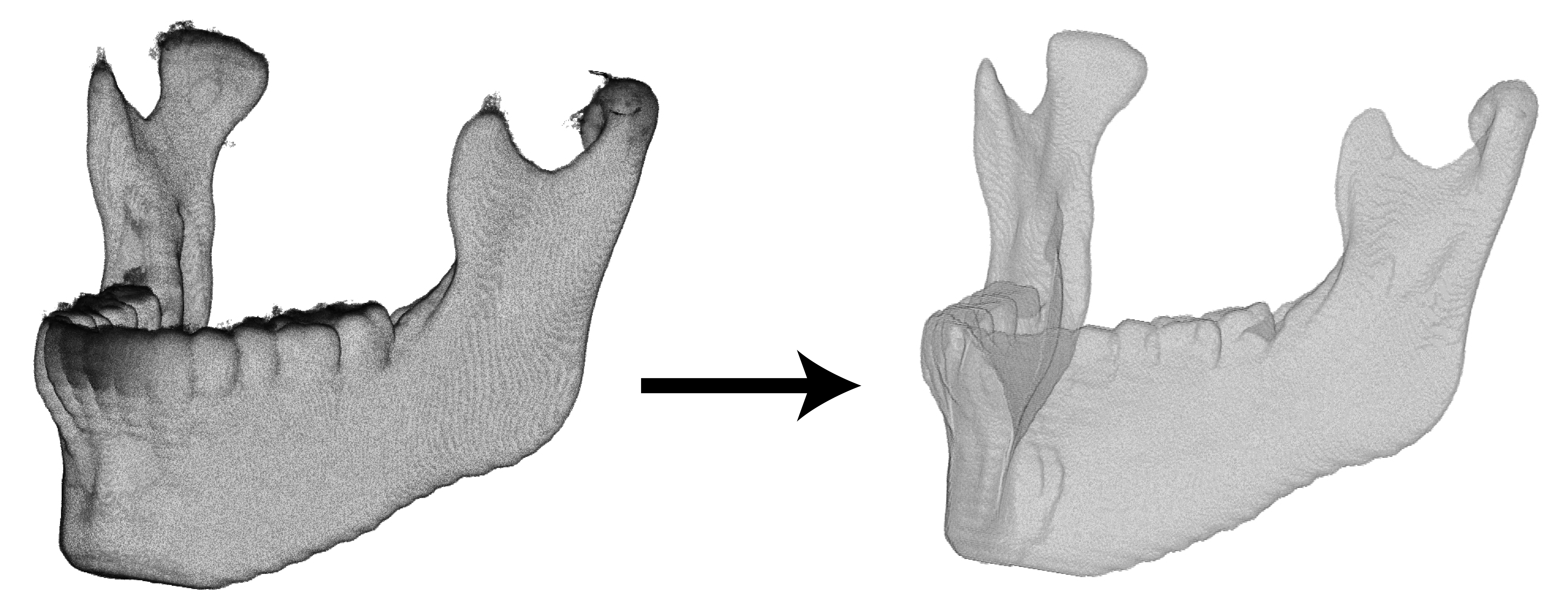
Left: Normalized mandible binary after compositing all 54 mandible binaries from registration processes. Mandibles are rendered on a grayscale here. Darker color represents low voxel/overlap intensity while lighter color represents high voxel/overlap intensity; Right: Mandible composite after normalization and threshold.

Note

3D Mandibles in figure above was rendered using the Volume Viewer module in ImageJ.

Post-processing

Once all compositing and averaging are completed, a single final composite mandible is generated. This composite mandible is viewed in MATLAB to determine if further manual touch-up is needed. In our case, the output from step 2 is in NIfTI file format so the load_nii function from the Tools for NIfTI and ANALYZE image package on MathWorks File Exchange is used to load accordingly

nii = load_nii('<allModels>.nii.gz')
mandible = isosurface(nii.img,0.5)

Now you can view the 3D mandible:

p = patch(mandible)
set(p,'FaceColor','<ColorValues>','EdgeColor','none')
camlight

3D mandible model rendered in MATLAB using a color matrix value of [0.75 0.75 0.70].

Rotate the mandible to inspect any regions requiring further enhancement

For more MATLAB parameters and specifications, refer to MATLAB documentation on Patch Properties.

Manual Editing

If the mandible needs to be edited manually, the NIfTI file will be padded into its original dimension using AFNI. Once padded, the mandible will be imported back into Analyze 12.0 for manual editing.

The following are used only if the user is using Analyze 12.0 as the editing software.

The padding values needed here are values recorded during pre-processing’s cropping step:

$ 3dZeropad -I <zlower> -S <zupper> -P <ylower> -A <yupper> -L <xlower> -R <xupper> -prefix <outputName> <allModels>.nii.gz
$ 3dAFNItoANALYZE <outputName> <outputName>+orig

When reloading the scan into the Analyze, users should flip the scan in X direction.